9.4. Running MD with GROMACS
9.4.1. DP/MM Simulation
This part gives a simple tutorial on how to run a DP/MM simulation for methane in water, which means using DP for methane and TIP3P for water. All relevant files can be found in examples/methane.
9.4.1.1. Topology Preparation
Similar to QM/MM simulation, the internal interactions (including bond, angle, dihedrals, LJ, Columb) of the region described by a neural network potential (NNP) have to be turned off. In GROMACS, bonded interactions can be turned off by modifying [ bonds ], [ angles ], [ dihedrals ] and [ pairs ] sections. And LJ and Columb interactions must be turned off by [ exclusions ] section.
For example, if one wants to simulate ethane in water, using DeepPotential for methane and TIP3P for water, the topology of methane should be like the following (as presented in examples/methane/methane.itp):
[ atomtypes ]
;name btype  mass  charge ptype    sigma  epsilon
  c3    c3   0.0     0.0     A 0.339771 0.451035
  hc    hc   0.0     0.0     A 0.260018 0.087027

[ moleculetype ]
;name            nrexcl
 methane          3

[ atoms ]
; nr type  resnr residue atom  cgnr  charge   mass
  1   c3      1     MOL   C1     1 -0.1068 12.010
  2   hc      1     MOL   H1     2  0.0267  1.008
  3   hc      1     MOL   H2     3  0.0267  1.008
  4   hc      1     MOL   H3     4  0.0267  1.008
  5   hc      1     MOL   H4     5  0.0267  1.008

[ bonds ]
; i  j  func  b0  kb
 1  2     5
 1  3     5
 1  4     5
 1  5     5

[ exclusions ]
; ai  aj1  aj2  aj3  aj4
  1    2    3    4    5
  2    1    3    4    5
  3    1    2    4    5
  4    1    2    3    5
  5    1    2    3    4
For comparison, the original topology file generated by acpype will be:
; methane_GMX.itp created by acpype (v: 2021-02-05T22:15:50CET) on Wed Sep  8 01:21:53 2021

[ atomtypes ]
;name   bond_type     mass     charge   ptype   sigma         epsilon       Amb
 c3       c3          0.00000  0.00000   A     3.39771e-01   4.51035e-01 ; 1.91  0.1078
 hc       hc          0.00000  0.00000   A     2.60018e-01   8.70272e-02 ; 1.46  0.0208

[ moleculetype ]
;name            nrexcl
 methane          3

[ atoms ]
;   nr  type  resi  res  atom  cgnr     charge      mass       ; qtot   bond_type
     1   c3     1   MOL    C1    1    -0.106800     12.01000 ; qtot -0.107
     2   hc     1   MOL    H1    2     0.026700      1.00800 ; qtot -0.080
     3   hc     1   MOL    H2    3     0.026700      1.00800 ; qtot -0.053
     4   hc     1   MOL    H3    4     0.026700      1.00800 ; qtot -0.027
     5   hc     1   MOL    H4    5     0.026700      1.00800 ; qtot 0.000

[ bonds ]
;   ai     aj funct   r             k
     1      2   1    1.0970e-01    3.1455e+05 ;     C1 - H1
     1      3   1    1.0970e-01    3.1455e+05 ;     C1 - H2
     1      4   1    1.0970e-01    3.1455e+05 ;     C1 - H3
     1      5   1    1.0970e-01    3.1455e+05 ;     C1 - H4

[ angles ]
;   ai     aj     ak    funct   theta         cth
     2      1      3      1    1.0758e+02    3.2635e+02 ;     H1 - C1     - H2
     2      1      4      1    1.0758e+02    3.2635e+02 ;     H1 - C1     - H3
     2      1      5      1    1.0758e+02    3.2635e+02 ;     H1 - C1     - H4
     3      1      4      1    1.0758e+02    3.2635e+02 ;     H2 - C1     - H3
     3      1      5      1    1.0758e+02    3.2635e+02 ;     H2 - C1     - H4
     4      1      5      1    1.0758e+02    3.2635e+02 ;     H3 - C1     - H4
9.4.1.2. DeepMD Settings
Before running simulations, we need to tell GROMACS to use DeepPotential by setting the environment variable GMX_DEEPMD_INPUT_JSON:
export GMX_DEEPMD_INPUT_JSON=input.json
Then, in your working directories, we have to write input.json file:
{
    "graph_file": "/path/to/graph.pb",
    "type_file": "type.raw",
    "index_file": "index.raw",
    "lambda": 1.0,
    "pbc": false
}
Here is an explanation for these settings:
graph_file: The graph file (with suffix .pb) generated bydp freezecommandtype_file: File to specify DP atom types (in space-separated format). Here,type.rawlooks like
1 0 0 0 0
index_file: File containing indices of DP atoms (in space-separated format), which should be consistent with the indices’ order in .gro file but starting from zero. Here,index.rawlooks like
0 1 2 3 4
lambda: Optional, default 1.0. Used in alchemical calculations.pbc: Optional, default true. If true, the GROMACS periodic condition is passed to DeepMD.
9.4.1.3. Run Simulation
Finally, you can run GROMACS using gmx mdrun as usual.
9.4.2. All-atom DP Simulation
This part gives an example of how to simulate all atoms described by a DeepPotential with Gromacs, taking water as an example. Instead of using [ exclusions ] to turn off the non-bonded energies, we can simply do this by setting LJ parameters (i.e. epsilon and sigma) and partial charges to 0, as shown in examples/water/gmx/water.top:
[ atomtypes ]
; name      at.num  mass     charge ptype  sigma      epsilon
HW           1       1.008   0.0000  A   0.00000e+00  0.00000e+00
OW           8      16.00    0.0000  A   0.00000e+00  0.00000e+00
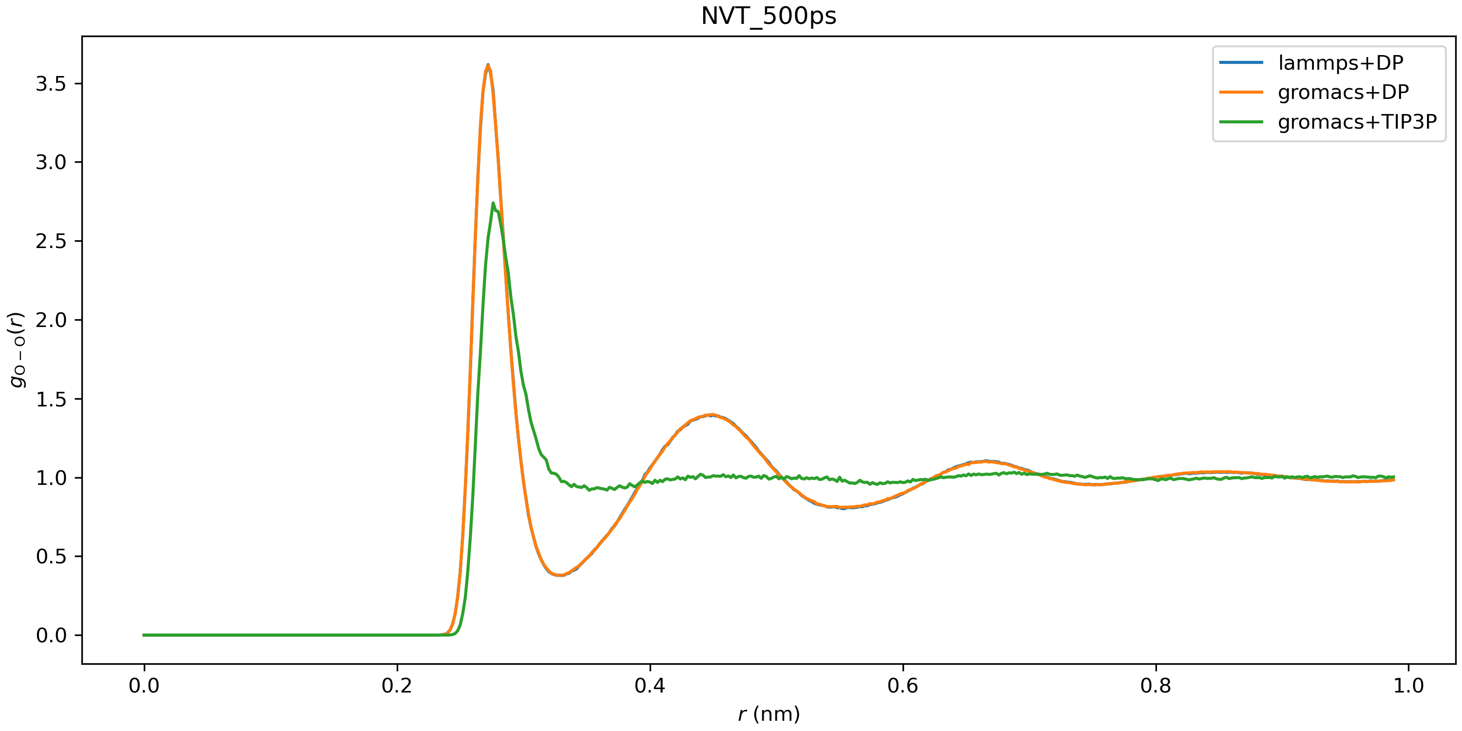
As mentioned in the above section, input.json and relevant files (index.raw, type.raw) should also be created. Then, we can start the simulation under the NVT ensemble and plot the radial distribution function (RDF) by gmx rdf command. We can see that the RDF given by Gromacs+DP matches perfectly with Lammps+DP, which further provides an evidence on the validity of our simulation. 
However, we still recommend you run an all-atom DP simulation using LAMMPS since it is more stable and efficient.